Category Archives: General

Fast Flexible Paxos

It’s official! Fast Flexible Paxos: Relaxing Quorum Intersection for Fast Paxos, my latest collaboration with Aleksey Charapko and Richard Mortier will appear in next year’s edition of the International Conference on Distributed Computing and Networking (ICDCN). If you don’t want to wait, then the paper is available right now on Arxiv and in the next few paragraphs, I’ll explain why I think this short paper opens the door to some exciting new directions for the future of high-performance state machine replication protocols. 

State machine replication

State machine replication (aka SMR) is a widely used technique for building strongly consistent, fault-tolerant services by replicating an application’s state machine across a set of servers and ensuring that each copy of the state machine receives the same sequence of operations. This is the primary responsibility of an SMR protocol such as Paxos, Chubby, Zookeeper[1] or Raft. SMR protocols are often criticized for performing poorly. Typically distributed systems opt for weaker consistency guarantees and reserve state machine replication only for the most critical aspects of a system such as managing metadata, distributed locking or group membership. 

Most SMR protocols take a similar approach to deciding the order that operations are applied to the state machines. They elect one server to be a leader and all operations for the state machines are sent first to the leader. The leader decides what order operations will be applied. Before the leader can apply an operation to its state machine, it first replicates it to a majority of servers to back up the operation. The leader can then safely apply the operation to its state machine. If the leader fails, then another server is chosen to become the new leader. A new leader must ensure that it knows about all operations which were applied by the failed leader. Since the previous leader replicated all applied operations to a majority of servers, the next leader can learn of all previously applied operations by communicating with the majority of servers. This is because any two majorities will overlap by at least one server.

In practice, it takes a while for an SMR protocol to apply an operation to the state machine. There are two main issues: firstly, all operations must be sent to the leader and secondly, all operations must then be replicated on a majority of servers. 

Fast Paxos

Various SMR protocols have been proposed to overcome the leader bottleneck. Some allow any server to directly replicate operations, without first sending them to the leader. I will refer to this as fast replication. The first protocol to support fast replication was Fast Paxos, which was proposed by Leslie Lamport in 2005. 

One downside of fast replication is that when a server replicates an operation, it now needs to make more copies before it is safe to apply the operation. Fast Paxos requires approximately 3/4 of servers to have a copy of an operation before it can be applied [2]. Fast Paxos might have handled one issue, the leader bottleneck, but in doing so, we have made the other issue even worse, we now need around 1/4 more copies of an operation before it can be applied.[3]

Flexible Paxos

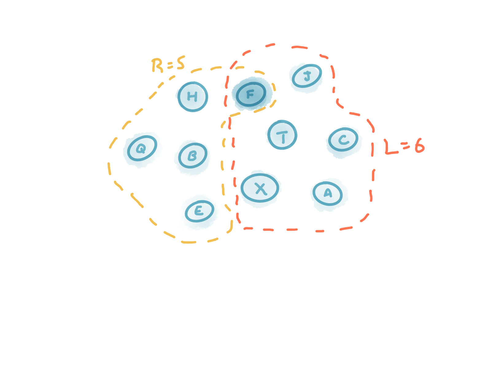
Regarding the issue of majority replication, Flexible Paxos showed that leaders could safely replicate operations to fewer servers, provided that more servers were used during leader election. The equation below describes the tradeoff between the number of servers which must participate in replication (R), the number of servers which must participate in leader election (L) and the total number of servers (N).

L + R > N 

Since leader election is rare, it benefits performance to reduce the number of servers which must replicate operations (R)  at the expense of increasing the number of servers which must participate in leader election (L).

For example, if N=10 then we might use R=5 and L=6.

Or we might choose to use R=3 and L=8.

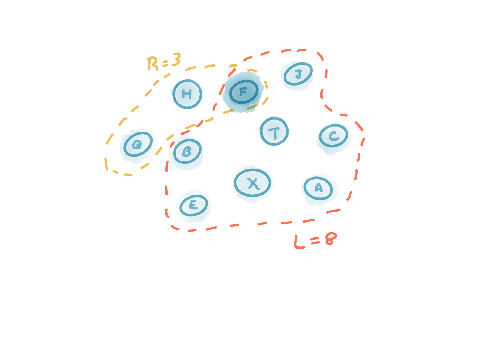
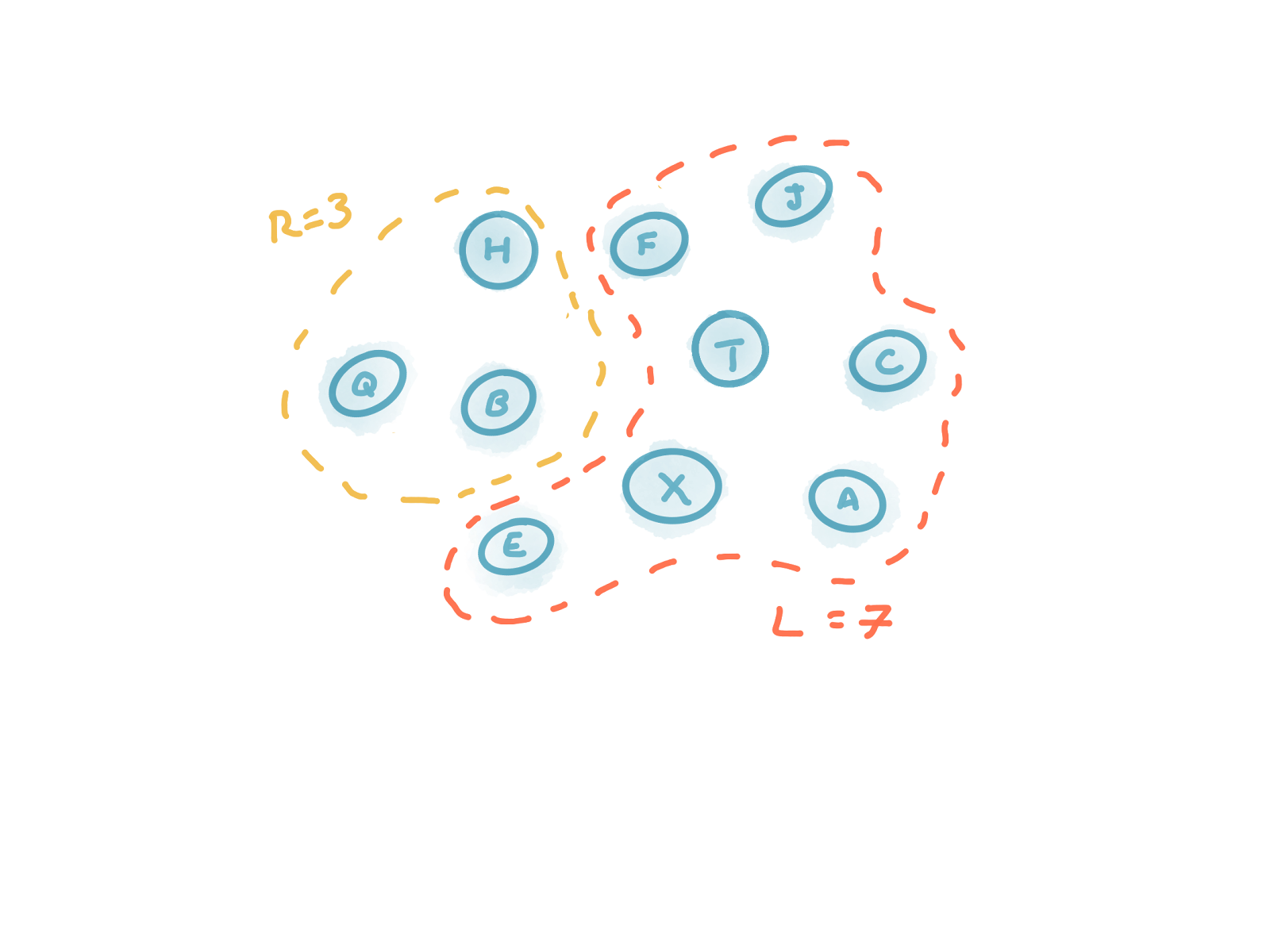
Note that we could not use R=3 and L=7. Our equation ensures that L and R always overlap by at least one server.

Fast Paxos + Flexible Paxos = Fast Flexible Paxos

Unfortunately, Flexible Paxos does not directly apply to Fast Paxos. State machine replication protocols thus need to choose between using a leader and requiring fewer copies of operations (Flexible Paxos) or allowing servers to bypass the leader but requiring more copies of operations (Fast Paxos). In this short paper, we prove that the approach of Flexible Paxos can be applied to Fast Paxos. Fast Paxos can safely replicate operations to fewer servers. We call this Fast Flexible Paxos.

Like Flexible Paxos, Fast Flexible Paxos observes that we can tradeoff the number of servers which replicate operations and participate in leader elections. The equations below describe this tradeoff in terms of R, L, N and the number of servers which must participate in fast replication (F).

L + R > N 

L + 2F > 2N

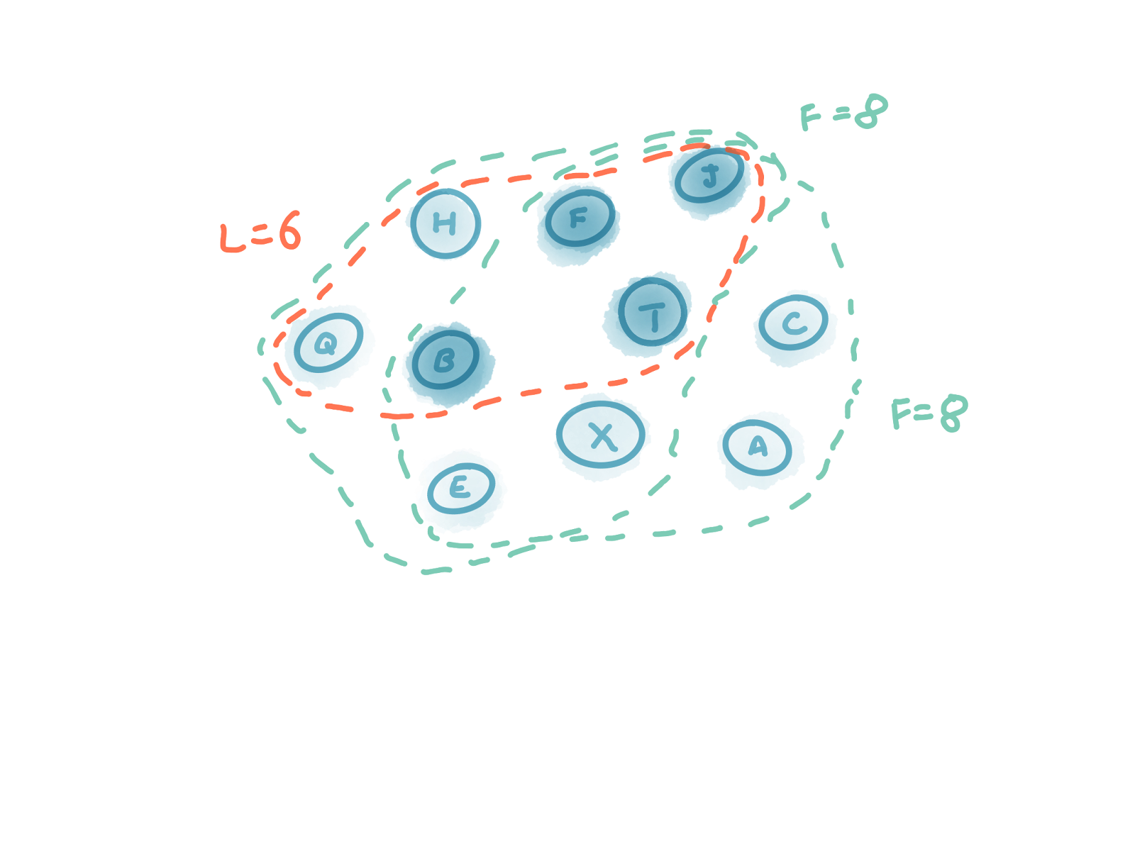
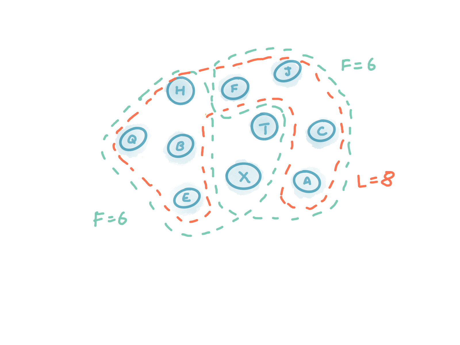
Consider the previous example where N=10, R=5 and L=6, our second equation requires that F=8.

Or consider the example where N=10, R=3 and L=8, this requires that F=7.

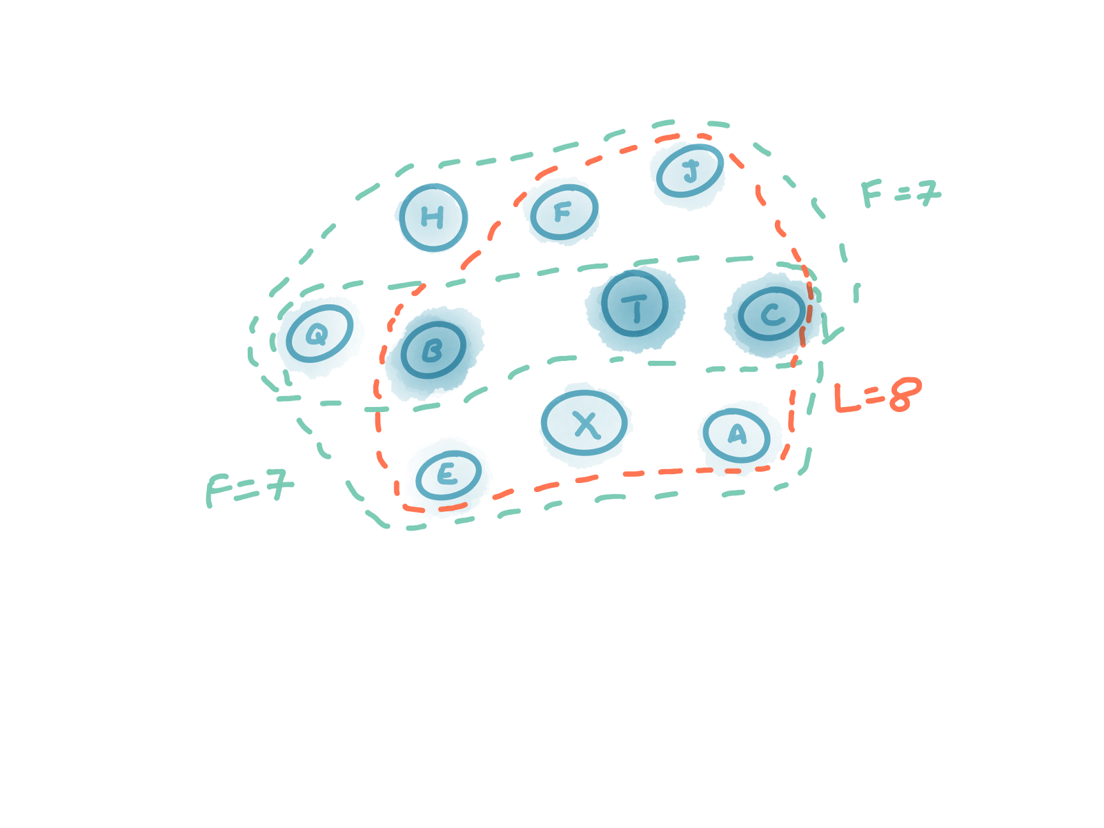
Note that it would not be ok to use N=10, L=8 and F=6, regardless of the value of R, as this does not satisfy our second equation. The second equation ensures that L always overlaps with any pair of Fs, as shown in the diagrams below.

As always with distributed systems, it is a matter of tradeoffs. In the most extreme case, we can use majorities for fast replication in Fast Flexible Paxos but this will not be able to tolerate any failures as it requires that L=N if N is odd.

Our paper on Fast Flexible Paxos describes exactly how we calculated these equations. The paper also includes a proof of Fast Flexible Paxos, a formal specification of Fast Flexible Paxos written in TLA+ and a prototype using Paxi.

State machine replication is a powerful primitive for distributed systems, which has the power to provide the strongest possible consistency guarantees even in the face of message delays and failures. However, the performance limitations of state machine replication have long limited its adoption. I believe that Fast Flexible Paxos is the first step towards building more performant state machine replication protocols which can support fast replication, thus addressing the leader bottleneck, without requiring most servers to participate in replication.

[1] Strictly speaking, Zookeeper uses atomic broadcast and primary backup replication but the same high-level ideas apply to both.

[2] ¾ is only required to tolerate the same number of failures as Paxos with majorities.

[3] There is another issue with fast replication which is that conflicts can occur when multiple servers try to replicate different operations at the same time. Subsequent protocols like Generalized Paxos and Egalitarian Paxos mitigate this.

Paper Notes on PBFT [OSDI’99]

Practical Byzantine Fault Tolerance (PBFT) is the foundational paper in Byzantine consensus algorithm. Typically, distributed consensus algorithms assume nodes may fail (and possible recovery), but BFT extends this to tolerate nodes acting arbitrarily.

Assumptions

BPFT makes strong assumption about these arbitrary failures. Notability that at most f failures will occur in a system of 3f+1 nodes, this bound applies to both safety and progress guarantees. In contrast, in typical paxos style consensus algorithms the bound of f failures in 2f+1 node only applies to progress guarantee, safety will always be guaranteed even if the system is not able to make progress. BPFT makes the usual asynchronous assumption, common to many consensus algorithms.

Algorithm

Section 4.2 describes the algorithm in details, the core idea is that once the nodes have been made aware of the request for a given log index, they under go a two step process where each node notifies every one of their agreement and proceed when at least f+1 nodes in the 2f+1 responses also agree. At end of the second stage, the client can be notified. Likewise, the view change protocol is a similarly enhanced version of view change from VRR.

Performance

BPFT takes 1.5 RRTs to commit a request in the common case, all requests must reach the system via a master node and after this time, all nodes have knowledge that the request was committed. In contract, typical multi-paxos algorithms (e.g., Raft and VRR) take 1 RTT to commit a request in the common case, again all requests must go via a master node but after this time only the master node has knowledge that the request was committed. Typical leaderless consensus algorithm (e.g., single-valued paxos) take at least 2 RTT to commit a request but requests can be submitted to any node. All cases we exclude the RTT from the client to the system node and back.

BPFT differs from typical consensus algorithms in the number of messages exchanged. Whilst there exists many optimizations to piggyback messages and reduce message load, we can approximate estimate of number of messages for algorithms (this time we are including client communication). A typical multi-paxos algorithms, might send 2n+2 messages for a commit in a system of n nodes, whereas BPFT might send 1 + 2n + 2n^2, a significant difference.

Conclusions

PBFT in an interesting read and an excellent contribution to consensus. However, I am not sure how common it is that a modern datacenter might meet assumptions laid out by the paper, in particular that at most f nodes might be faulty in a system 3f+1 nodes. In this environment, nodes are usually running a same OS, configurations, software stacks and consensus implementation. Thus if an adversary is able compromise a machine then it’s likely they can compromise many, thus failures are very much dependent on each other. Lets see if the 17 years of research since has been able to improve on this.

BBC Radio 4: Any questions?

I asked a question on today’s BBC radio 4 show “Any questions?”, http://www.bbc.co.uk/programmes/b06b3ny4, skip to 42:07 to hear me nervously ask “How can we protect the rights of citizens in an increasingly digital world?” and hear the panel’s response. The responses where fairly disappointing but it helps to keep the debate alive.

Azure Latency Pilot Study: Part 3 – Machine specific results

In this post we will be looking at the results for the Azure latency Pilot study described last week. Yesterday, we started by looking at the aggregated results and found that the measured RTT was larger then expected. Today, we will look at how the results vary depending on which VMs the measurements where taken between. It may be the case that we can infer something about topology between VMs, for example whether VM’s are in the same physical host and the same rack.

The table below shows the RTT between each pair of VMs. The first server in the pair, labelled src is the one which initialised the ping. The table includes each machine pinging itself for comparison.

src dst mean s.d min 25th 50th 75th max
1 1 51.0 65.1 1.7 4.3 65.25 71.6 1004.0
1 2 12.1 89.7 1.7 2.9 3.6 4.3 1004.7
1 3 9.5 66.5 1.6 3.4 4.1 4.8 1004.7
1 4 7.3 52.3 1.3 3.0 3.5 4.0 1004.1
1 5 11.8 84.9 1.6 3.0 3.6 4.4 1242.2
2 1 6.2 12.7 1.6 3.0 3.7 4.425 88.4
2 2 16.7 65.8 1.1 3.0 3.7 4.6 1002.9
2 3 15.0 95.6 1.4 3.0 3.7 4.4 1004.9
2 4 9.6 62.0 1.4 2.9 3.5 4.3 1003.6
2 5 15.3 80.0 1.3 2.9 3.5 4.3 1002.5
3 1 48.5 44.9 2.0 4.5 64.2 70.6 754.9
3 2 7.0 48.9 1.4 2.9 3.6 4.4 1005.0
3 3 3.9 4.2 1.6 3.1 3.8 4.6 124.9
3 4 5.8 32.0 1.3 2.9 3.4 4.0 628.6
3 5 6.7 52.5 1.5 2.9 3.8 4.4 1229.3
4 1 48.8 48.3 1.9 4.7 62.1 67.3 1003.0
4 2 7.7 59.5 1.3 2.8 3.6 4.4 1003.8
4 3 9.0 60.1 1.6 3.3 4.1 4.8 1004.0
4 4 5.2 29.3 1.2 2.7 3.3 3.8 754.6
4 5 15.6 104.7 1.5 2.8 3.6 4.3 1035.0
5 1 50.9 69.8 2.0 4.5 63.8 69.6 1005.3
5 2 9.4 70.9 1.3 2.9 3.7 4.3 1003.8
5 3 8.6 57.6 2.0 3.3 4.1 4.8 1003.7
5 4 6.5 47.7 1.3 2.7 3.4 4.0 1003.0
5 5 6.8 49.2 1.2 2.5 3.2 4.1 1023.0

All VMs other than VM 2 have high latency to VM 1. In fact, we see an average 65 ms RTT from VM 1 to itself. This warrants further investigation into how hping3 is measuring latency. Removing VM 1 from the equation, we observe reasonable uniformity in the RRTs between VMs 2 to 5. Between these the min, 25th, 50th and 75th percentile are all similar and the maximum varies highly, which is to be expected.

I would like to take a close look at how the distribution of RTT measurements varies between VMs 2 to 5. The table below shows the RTT between each pair of VMs between 2 to 5, at various percentile points.

src dst 80th 90th 95th 98th 99th
2 2 5.1 41.8 47.2 124.6 150.7
2 3 4.6 5.0 5.5 34.5 429.5
2 4 4.5 4.9 5.5 47.4 78.5
2 5 4.5 5.4 60.4 91.8 207.8
3 2 4.5 4.8 5.0 5.5 8.9
3 3 4.7 5.0 5.1 5.4 5.8
3 4 4.2 4.5 4.8 5.2 6.1
3 5 4.6 4.9 5.2 5.9 6.6
4 2 4.5 4.8 5.0 5.2 5.8
4 3 5.0 5.2 5.4 5.7 6.4
4 4 4.0 4.3 4.7 5.1 5.8
4 5 4.5 4.8 5.2 6.1 762.9
5 2 4.5 4.8 4.9 5.1 6.1
5 3 4.9 5.2 5.4 5.6 6.8
5 4 4.1 4.5 4.9 5.3 6.3
5 5 4.3 4.6 4.8 5.8 7.2

Yesterday, we saw that the 90th percentile for dataset as a whole was 61.4 ms, this is not representative of the RTT between VMs 2-5. We can see this information more clearly using the following 5 CDF, each graph representing the round trip time from each machine to each of the others (and itself).

alt text
alt text
alt text
alt text
alt text

Machine 1 is a clear outlier from the perspective for machines 1, 3, 4 and 5. The observed RTT doesn’t seems to be symmetric. Again this asymmetry warrants further investigation. The stepping in the CDFs is because the RTT is recorded to the nearest 1 decimal place.

Next time, we will look at how the observed RTT varies with time.

Azure Latency Pilot Study: Part 2 – Aggregated results

This is post we will be looking at the results for the Azure latency Pilot study described last week. We will starting by looking at the aggregate results, disregarding the time a measurement was taken and which machines the measurement was taken between.

The 22332 data points have been processed in Python3, in particular using the matplotlib and numpy libraries. The scripts are available in azure-measurements repository.
They currently only use the average round trip time, as reported by hping3, average over 10 pings.

property RTT (ms)
min 1.1
max 1242.2
mean 15.9
std 66.5

The results in the table above are much larger than I expected. Given the large standard deviation and very large maximum value, it is likely that a few large measures have skewed the results. Let’s take a look at the cumulative distribution function (CDF) and percentile points to see if this is the case.

percentile RTT (ms)
25th 3.0
50th 3.8
75th 4.7
90th 61.4
95th 69.7
99th 87.3

alt text

As expect, some large measurements have skewed the results. However, the proportion of measurement which are considered large is much greater then I expected. This warrants further investigation.

Before that, lets take a closer look at how the majority of value are distributed. Due to the central limit theorem and the sufficiently large sample size, we would expect to see a normal distribution. In simulators such as Raft Refloated, we simulate latency as normally distributed with given parameters, discarding values below a threshold value. We can take a closer look at the probability density function (PDF) and see if this is a reasonable approximation.

alt text

The green bars represent the probability of each RTT. We see an approximate normal distribution, although it is clear that this distribution doesn’t have the same parameters as the data set as a whole. The red lines shows a normal distributed with mean 3.6 and standard deviation of 1. This red line appears to be a reasonable approximation and could be used in simulation.

Next post, we will looks at how the measured RTT differs depending which of the 5 machines the measurement was taken between.