Do you want a shed or a castle?

I have seen the error of my (programming) ways. Let me explain…

To me, programming in OCaml is like trying to build a house from just breeze blocks. It takes a long time to build even a simple shed. However. when its done, its really quite solid.

To me, programming in Go is like building a house from an array of complex pre-build components. In the blink of an eye, you have an amazing castle, complete with turrets and ornate window frames.

You open the door to your beautiful new castle and it all fails down. Each time you rebuild one part, another falls down.

You are full of regrets as you sleep in the wreckage of your fallen castle and wish for a solid shed.

Another fallen castle – rod collier [CC BY-SA 2.0 (http://creativecommons.org/licenses/by-sa/2.0)], via Wikimedia Commons

Yours truly,

Someone fighting to hold up a fallen castle

EDIT: here’s  some more example of what a falling castle looks like

Screen Shot 2016-04-28 at 14.46.46

Screen Shot 2016-04-28 at 14.52.34

Speaking at QCon London 2016

I am pleased to announce that I’ll be speaking at this year’s QCon London. I’ll be speaking in the “Modern CS in the real world” track, hosted by none other than Adrian Colyer, from the morning paper.  The abstract for my talk,  Making the Impossible Possible is as follows:

In this talk, we explore how to construct resilient distributed systems on top of unreliable components.

Starting, almost two decades ago, with Leslie Lamport’s work on organising parliament for a Greek island. We will take a journey to today’s datacenters and the systems powering companies like Google, Amazon and Microsoft. Along the way, we will face interesting impossibility results, machines acting maliciously and the complexity of today’s networks.

Ultimately, we will discover how to reach agreement between many parties and from this, how to construct new fault-tolerance systems that we can depend upon everyday.

The talk will be based upon the material from my master lecture, Reaching reliable agreement in an unreliable world. The slides for which are online and below.

Paper Notes on “CORFU: A distributed shared log” [TOCS’13]

Last Monday we looked at Tango, a system for replicating a data structure to provide linearizable semantics and fault-tolerance. Tango is built up on CORFU, a replicated log, built over storage nodes. This paper notes article covers “CORFU: A distributed shared log” also by Balakrishnan et al. from TOCS December 2013. I believe that this paper elaborates on “CORFU: A Shared Log Design for Flash Clusters” by Balakrishnan et al from NSDI 2012 and that the NSDI paper is not a prerequisite for the TOCS paper.

What we already know?

From the Tango paper, we learned that CORFU provides a replicated log with support for the following operations: append, check, read, trim and fill.

Its main two components are: a sequencer, which hands out addresses in the log and storage nodes (such as SSDs) which store log entries. Storage nodes are divided into clusters and a variant of chain replication is used between them. Each cluster is responsible for a subset of log addresses.

Summary

This paper presents CORFU, a shared log, distributed over storage nodes. It main advantage over existing systems is its scalability as its not bottlenecked by the I/O of a single host.

Local addresses -> physical addresses

Each storage node exposes a infinite write-once logical address space with read, write, delete and fill operations for each address. Delete is used when the data at a particular logical address is not longer required, its physical address can be reused but its logical address cannot. Fill is used to mark that a logical address will not be used in the future. These are implemented using a hash table with various optimizations. A seal operations is also provided which locks a storage node to operates with equal or higher epoch number.

Global addresses -> local addresses

Each client resolves a global address into a set of nodes and a local address in two stages. Firstly, the client uses a local copy of a mapping from ranges in the global addresses space to disjoint subsets of hosts. For example, addresses 0-100K map to replica sets A-C and addresses 100K-200K map to replica sets D-F. A deterministic function (like mod and div) maps the specific global address to a local address a specific replica set like A or C.

Replication

Replica are written to using client-driven chain replication, this means the client writes to each replica in a deterministic order and waits for successful acknowledgment for each storage node before continuing. As a result, write latency scales linearly with the number of replicas. In contrast, majority-based protocol like Raft, Paxos and VRR can replicate a write in as little as 1 RTT, regardless of the number of nodes, in the right conditions. The downside of such protocols is that to tolerant f failure we need 2f+1 nodes instead of f+1.

If a client fails to complete this process then it may be filled in by the next client. Like Raft, this means that clients may be given false negatives, and thus the application utilizing the log must be able to handle this. For example, Raft uses operation id’s and caches to prevent multiple application of the same operation to a state machine in SMR.

A more important failure case is where a client fails to see a committed write since the replica it is querying was removed from the replica set due to network partition/failure and the client is not aware of this change. This is address by issuing leases to the storage units from the sequencer.

Changing projections

Corfu’s sequencer is in some ways analogous to the coordinator/master in tradition protocols. Likewise, Corfu’s changing projection has many parallels with VRR’s view changes or Raft’s term changes. In all cases, a monotonically increasing value (known as the epoch number/view number/term) separates different perspectives on system configuration. Example prospectives include a period of leadership in Raft or a set of projections in CORFU. Each node stores its prospective of this value and each message between nodes includes it. Projection change is initiated by a client, then agreed by storage nodes using a Paxos-like consensus protocol and then each (involved) storage node is sealed in the process. Clients learn of the projection change when they contact storage nodes (since it includes their outdated epoch) and they retrieve the new projection information from a networked storage drive.

My interpretation of changing projections is that each projection change can include a completely new configuration. This mechanism provides us with dynamic membership, in addition to a mechanism for dealing with network failures and partitions.

Evaluation

The authors’ experimental evaluation seems very promising. In some ways, it is difficult for me to determine which gains are from the hardware and which are from CORFU’s design. All of the experiments use two replicas per cluster, thus just two failures are capability of bringing the system down. The use of client-driven chain replication means that I would really like to see how the system scales (particularly its latency) with more replicas.

Conclusions

Corfu is a very interesting system and seems to be a novel point on the solution space of distributed log solutions. Next time, we will take a look at the open source implementation, CorfuDB.

Paper Notes on “Tango: Distributed Data Structures over a Shared Log” [SOSP’13]

The following is a paper notes article on “Tango: Distributed Data Structures over a Shared Log” by Balakrishnan et al. from SOSP 2013. The article focus on the main body of the paper and I will cover Tango’s streaming and transaction support in a separate article, sometime in the future.

I have covered this paper before covering its companion paper “CORFU: A Shared Log Design for Flash Clusters” also by Balakrishnan et al. from NSDI 2012. I expect its paper notes article will answer many of the open questions in this article.

Summary

Tango is system for replicating a data structure to provide linearizable semantics and fault tolerance. Tango is framed as system for application metadata, whose requirement include a need for fault tolerance, high availability, fairly strong consistency/ordering requirements.

[quick note on terminology: unlike the usual terminology to describe systems like Raft and VRR, Tango uses the term “client” to refer to what similar systems call a server and “external client” to what similar systems call a client. We shall use the same terminology as Tango. ]

The basics

At its heart, Tango, takes SMR and separates the replication of the log from the hosts running the application. In traditional SMR, each host runs the application itself (an in-memory deterministic state machine) and stores a local copy of the log. With the help of a consensus protocol, the local copy of the log kept upto date and clients are provided with linearizable semantics. In Tango, only the application runs on these host. The log is instead distributed (using chain replication) across an a set of storage nodes (e.g. an SSD cluster). Tango clients do not communicate directly with message passing (as is the case of SMR), instead they interact via the shared log.

SMR is often used with leader driven consensus, this means that only the leader may commit an operation to replicated log and if the leader was to fail the system is unavailable to clients until a new leader is chosen. In contrast, Tango’s approach allows clients to directly replicate commands to the log. The leader is replaced by a dedicated sequencer and the sequencer state is soft so systems can continue to operate (at higher latency) if the sequencer was to fail.

Tango uses a stream abstraction to shard operations by the data structure on which they operate. This is used to clients to efficiently “ignore” operations which do not apply their data structures.

Shared log (aka Corfu)

The shared log (aka Corfu) is composed of clusters of storage nodes. Within each cluster, each storage node is a replica and operates on a read many/write once basis. Global address x maps to cluster (x mod n) and local address (x div n), where n is the number of clusters. Clients read and write to clusters using chain replication, this is also how failures are handled.

The sequencer stores the global address of the log tail. If this fails, it can reconstructed by querying storage nodes for local address of their log tail. The paper also mentions that each cluster also has its own dedicated sequencer, I could not understand when this is used.

Multiple clients writing to one address is resolved safely and Corfu exposes an operation for filling in unused addresses

Application interface

In many classic protocols, the external client must locate a master/coordinator to handle the request on their behalf. In Tango (like some other leaderless systems like EPaxos) any external client can communication with any client. Often SMR uses master leases or a similar mechanism to handle read requests without fully replicating them (unlike write requests) or having to pass them to the master. Corfu supports a check operation so Tango can check (and update if necessary) the local view before applying the update. Transactions are supported with speculation, object version numbers and a commit/abort stage before an up call to application is made

The API for interfacing with Tango seems similar to that of SMR. An application must provide a callback to apply a operation and has access to method to add read or write operations. An application may provide a checkpointing mechanism and may call discard on any log prefix.

Related systems

Alternatives to Tango are systems such as Zookeeper, Raft and Chubby. In the introduction, the authors highlight that such system are not sufficient since they only support specific data structures and/or do not support operations over multiple data structures. Whilst I support this idea, I would argue that in at least some existing systems, operations over multiple data structure can be supported by considering the multiple data structures as one. This allows operations over multiple data structure but comes at a high cost of adding a total ordering between operations when only a small partial ordering is required. Since Tango support streaming, it already has access to a partial ordering on operations instead of just using a total ordering. P-SMR by Parisa Marandi demonstrates the efficiently improvements possible by utilizing this information. Another argument given in the paper is that adopting SMR after the development of an application “often requires a drastic rewrite of the code”.

Evaluation

The experimental evaluation of Tango focuses on measuring throughput and/or latency whilst varying the number of clients and ratio of write to read requests. I would be interested to see some results on the recovery time for various patterns of storage node or sequencer failures. The initial evaluation considers three scenarios: (a) 18 storage nodes and 1 client, (b) 18 storage nodes and 2 clients, (c) 2 or 18 storage nodes and 1 to 18 clients. Generally speaking, the results are very much as you might expect: increasing request load increases request latency, writes place a much high burden on the system than reads and read only clients scale linearly until storage nodes are saturated.

The paper does not mention any formal proof of correctness (only that the sequencer is not required for correctness). Log compaction is supported with the forget call and checkpointing. Dynamic membership support for clients is trivial due to the design of Tango but I would be interested how Corfu and its variant of chain replication handles storage node failures.

It is not fair to directly compare Tango to systems using SMR with a majority quorum consensus algorithm (such as Raft). Tango’s scalability comes (in part) from the sharding of the replication log into clusters. This technique can be applied to SMR (see S-SMR) too. It would be interesting to see how Tango performs with the storage node, application node and sequencer co-located on same the host. However (particularly with current trend towards containers, docker and unikernels) separating systems like Tango into function specific instances/hosts has some significant benefits such as decoupling the number of storage and application hosts or fine gained provisioning for the sequencer compared to the storage/application hosts.

Conclusion

Each new paper that presents a high availability, fault-tolerance systems seems to build upon many of the old concepts (such as Paxos, SMR and timeouts for failure detection), in combination with a few novel ideas. In this case, Tango builds upon chain replication, for replicating log entries and the typical API for SMR. This is first time I have seen a soft state sequencer used in such as system as well as the divide between the storage nodes and application nodes. Overall, I really like this paper and its nice to see some novelty in a space crowded with variants of Paxos + SMR.

BBC Radio 4: Any questions?

I asked a question on today’s BBC radio 4 show “Any questions?”, http://www.bbc.co.uk/programmes/b06b3ny4, skip to 42:07 to hear me nervously ask “How can we protect the rights of citizens in an increasingly digital world?” and hear the panel’s response. The responses where fairly disappointing but it helps to keep the debate alive.

Azure Latency Pilot Study: Part 4 – Variation in results with time

So far in this study, we have only considered the aggregated measurements and how they vary depending on the VMs used. In this post, we will considered how the RTT measurements may have changed over time.

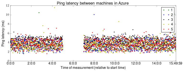
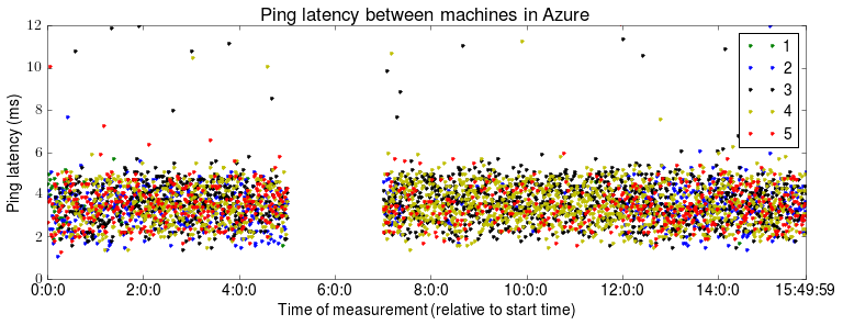
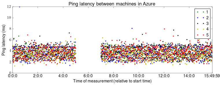
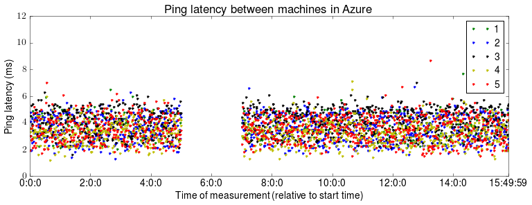
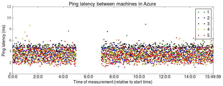
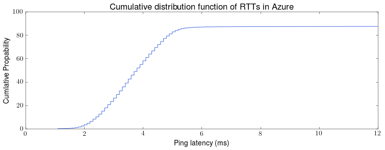
The following 5 plots show the RTT as observed by each machine over time. The y axis stops as 12 ms to aid visibility of the majority of results. Using the CDF of all results from the second part in this series, we can see that these figures thus include around 85% of all data points.

alt text
alt text
alt text
alt text
alt text

The most striking aspect of these figures is the 2 hour gap in the results. The source of this failure is still unknown. Azure reported no machine or network failures during this time and the system removed and continued to take measurements without any manual intervention. Otherwise, between 2 and 5 ms the RTT measurements appear to be fairly randomly distributed, although as we saw last time their distribution approximates normal (as we would expect).

Overall, I am not particularly happy with the results collected so far and hope the next round of tests will generate better results. Tomorrow, we will compare how these results differ from other studies.

Azure Latency Pilot Study: Part 3 – Machine specific results

In this post we will be looking at the results for the Azure latency Pilot study described last week. Yesterday, we started by looking at the aggregated results and found that the measured RTT was larger then expected. Today, we will look at how the results vary depending on which VMs the measurements where taken between. It may be the case that we can infer something about topology between VMs, for example whether VM’s are in the same physical host and the same rack.

The table below shows the RTT between each pair of VMs. The first server in the pair, labelled src is the one which initialised the ping. The table includes each machine pinging itself for comparison.

src dst mean s.d min 25th 50th 75th max
1 1 51.0 65.1 1.7 4.3 65.25 71.6 1004.0
1 2 12.1 89.7 1.7 2.9 3.6 4.3 1004.7
1 3 9.5 66.5 1.6 3.4 4.1 4.8 1004.7
1 4 7.3 52.3 1.3 3.0 3.5 4.0 1004.1
1 5 11.8 84.9 1.6 3.0 3.6 4.4 1242.2
2 1 6.2 12.7 1.6 3.0 3.7 4.425 88.4
2 2 16.7 65.8 1.1 3.0 3.7 4.6 1002.9
2 3 15.0 95.6 1.4 3.0 3.7 4.4 1004.9
2 4 9.6 62.0 1.4 2.9 3.5 4.3 1003.6
2 5 15.3 80.0 1.3 2.9 3.5 4.3 1002.5
3 1 48.5 44.9 2.0 4.5 64.2 70.6 754.9
3 2 7.0 48.9 1.4 2.9 3.6 4.4 1005.0
3 3 3.9 4.2 1.6 3.1 3.8 4.6 124.9
3 4 5.8 32.0 1.3 2.9 3.4 4.0 628.6
3 5 6.7 52.5 1.5 2.9 3.8 4.4 1229.3
4 1 48.8 48.3 1.9 4.7 62.1 67.3 1003.0
4 2 7.7 59.5 1.3 2.8 3.6 4.4 1003.8
4 3 9.0 60.1 1.6 3.3 4.1 4.8 1004.0
4 4 5.2 29.3 1.2 2.7 3.3 3.8 754.6
4 5 15.6 104.7 1.5 2.8 3.6 4.3 1035.0
5 1 50.9 69.8 2.0 4.5 63.8 69.6 1005.3
5 2 9.4 70.9 1.3 2.9 3.7 4.3 1003.8
5 3 8.6 57.6 2.0 3.3 4.1 4.8 1003.7
5 4 6.5 47.7 1.3 2.7 3.4 4.0 1003.0
5 5 6.8 49.2 1.2 2.5 3.2 4.1 1023.0

All VMs other than VM 2 have high latency to VM 1. In fact, we see an average 65 ms RTT from VM 1 to itself. This warrants further investigation into how hping3 is measuring latency. Removing VM 1 from the equation, we observe reasonable uniformity in the RRTs between VMs 2 to 5. Between these the min, 25th, 50th and 75th percentile are all similar and the maximum varies highly, which is to be expected.

I would like to take a close look at how the distribution of RTT measurements varies between VMs 2 to 5. The table below shows the RTT between each pair of VMs between 2 to 5, at various percentile points.

src dst 80th 90th 95th 98th 99th
2 2 5.1 41.8 47.2 124.6 150.7
2 3 4.6 5.0 5.5 34.5 429.5
2 4 4.5 4.9 5.5 47.4 78.5
2 5 4.5 5.4 60.4 91.8 207.8
3 2 4.5 4.8 5.0 5.5 8.9
3 3 4.7 5.0 5.1 5.4 5.8
3 4 4.2 4.5 4.8 5.2 6.1
3 5 4.6 4.9 5.2 5.9 6.6
4 2 4.5 4.8 5.0 5.2 5.8
4 3 5.0 5.2 5.4 5.7 6.4
4 4 4.0 4.3 4.7 5.1 5.8
4 5 4.5 4.8 5.2 6.1 762.9
5 2 4.5 4.8 4.9 5.1 6.1
5 3 4.9 5.2 5.4 5.6 6.8
5 4 4.1 4.5 4.9 5.3 6.3
5 5 4.3 4.6 4.8 5.8 7.2

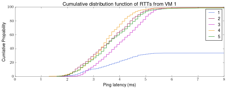
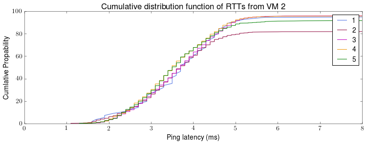
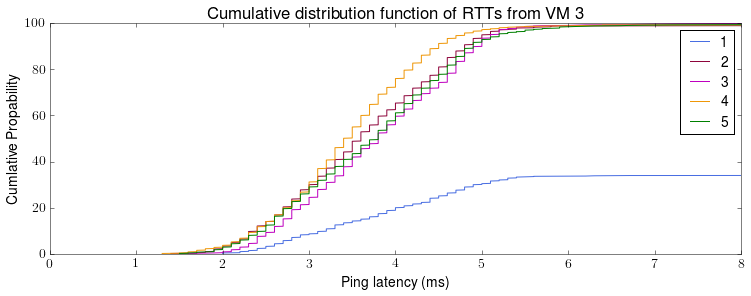
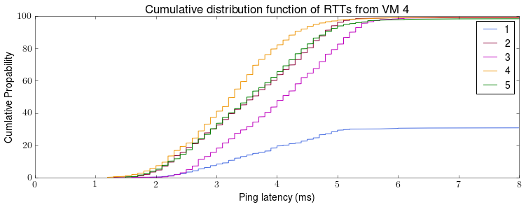
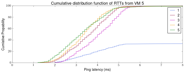
Yesterday, we saw that the 90th percentile for dataset as a whole was 61.4 ms, this is not representative of the RTT between VMs 2-5. We can see this information more clearly using the following 5 CDF, each graph representing the round trip time from each machine to each of the others (and itself).

alt text
alt text
alt text
alt text
alt text

Machine 1 is a clear outlier from the perspective for machines 1, 3, 4 and 5. The observed RTT doesn’t seems to be symmetric. Again this asymmetry warrants further investigation. The stepping in the CDFs is because the RTT is recorded to the nearest 1 decimal place.

Next time, we will look at how the observed RTT varies with time.

Azure Latency Pilot Study: Part 2 – Aggregated results

This is post we will be looking at the results for the Azure latency Pilot study described last week. We will starting by looking at the aggregate results, disregarding the time a measurement was taken and which machines the measurement was taken between.

The 22332 data points have been processed in Python3, in particular using the matplotlib and numpy libraries. The scripts are available in azure-measurements repository.
They currently only use the average round trip time, as reported by hping3, average over 10 pings.

property RTT (ms)
min 1.1
max 1242.2
mean 15.9
std 66.5

The results in the table above are much larger than I expected. Given the large standard deviation and very large maximum value, it is likely that a few large measures have skewed the results. Let’s take a look at the cumulative distribution function (CDF) and percentile points to see if this is the case.

percentile RTT (ms)
25th 3.0
50th 3.8
75th 4.7
90th 61.4
95th 69.7
99th 87.3

alt text

As expect, some large measurements have skewed the results. However, the proportion of measurement which are considered large is much greater then I expected. This warrants further investigation.

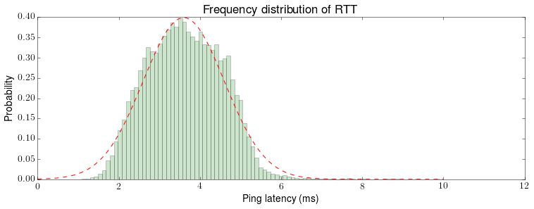
Before that, lets take a closer look at how the majority of value are distributed. Due to the central limit theorem and the sufficiently large sample size, we would expect to see a normal distribution. In simulators such as Raft Refloated, we simulate latency as normally distributed with given parameters, discarding values below a threshold value. We can take a closer look at the probability density function (PDF) and see if this is a reasonable approximation.

alt text

The green bars represent the probability of each RTT. We see an approximate normal distribution, although it is clear that this distribution doesn’t have the same parameters as the data set as a whole. The red lines shows a normal distributed with mean 3.6 and standard deviation of 1. This red line appears to be a reasonable approximation and could be used in simulation.

Next post, we will looks at how the measured RTT differs depending which of the 5 machines the measurement was taken between.

Azure Latency Pilot Study: Part 1 – Experimental Setup

This post, the first in a short series, discusses a simple overnight pilot study of measuring network characteristics on Microsoft Azure. This study was to be the first of many. Its purpose was to test the tools and gave some initial measurements, thus informing the the design of more substantial measurement studies in the future.

Motivation

Ultimately, I would like to answer the following questions about today’s cloud offerings:
1. How often do VMs fail in practice? What is the typical downtime? And to what extent are these failures correlated with each other? How does the failure rate vary with different price tiers and different cloud providers? For example, comparing normal instances to low cost instances like Amazon EC2 Spot instances or Google Clouds Preemptible Instances
2. How often do network partitions occur? What types of partitions do we see in practice? Do they isolate individual nodes or divide a cluster into a few disconnected groups? Do partial partitions, which we believe can cause issues for protocols such as Raft, occur in practice?
3. What are the latency characters between VMs? How about between between different datacenters by the same provider or by different providers?
4. How do today’s open source fault-tolerant data stores such as LogCabin or CorfuDB perform in practice? Is this sufficient to meet application demands? How quickly can such system heal after failures?
5. How can use the above to configure systems such as Raft Refloated or Coracle to simulate real work deployments of fault tolerance applications?

Experimental Setup

The experiment was run across virtual machines in the Azure. Azure is Microsoft’s cloud offering and a competitor to services such as Google Cloud and Amazon EC2. Azure was chosen simple over the competition simply because we have access to free credits. This was the first time I had used it (except from hosting the Coracle SIGCOMM demo) and it was relatively straight forward to perform simple operations, though not without its difficulties. For the management of the virtual machines, I mostly used Azure ASM CLI, a command line utility for managing VMs, its written in JS and is open source. This first test used 5 ‘small’ machines in North Europe, running overnight.

The machine themselves where simple Ubuntu 14.03 instance (and yes, Azure does have linux VM’s too). One machine was manually set-up, captured and cloned. Setup involved adding the public key of the data collection server, cloning measurement scripts and running them as a service, installing a few dependencies and running sudo waagent -deprovision before capturing the VM image.

Measurements

The measurement script simply TCP pings (sends SYN and waits for response) all the other machines in the test set every 20 sec and writes the results with test time to disk. It is worth noting that Azure drops ICMP traffic and whilst they acknowledge that is case of external traffic, many people (myself included) could not get internal ICMP traffic through either. The tool used was hping3, and it reported min, max and average round trip from a 10 successive pings.

The measurement server waited until after the end of the measurement study to collect data, to avoid interfering with the measurement. The collection script simply pulls the data from the measurement servers using scp (and the asymmetric keys established earlier). The other management jobs such as cleaning the data files or updating measurement scripts was done using parallel ssh.

Results

The experiment was ran between 19:00 and 08:50:00, across 5 virtual machines. In total, 22332 measurements were involved in the analysis, ranging from 1.1 ms to 1242 ms. The raw data is available online, as are all the scripts used.

Tomorrow, we will look at some analysis of these results.