Tag Archives: tw

Speaking at QCon London 2016

I am pleased to announce that I’ll be speaking at this year’s QCon London. I’ll be speaking in the “Modern CS in the real world” track, hosted by none other than Adrian Colyer, from the morning paper.  The abstract for my talk,  Making the Impossible Possible is as follows:

In this talk, we explore how to construct resilient distributed systems on top of unreliable components.

Starting, almost two decades ago, with Leslie Lamport’s work on organising parliament for a Greek island. We will take a journey to today’s datacenters and the systems powering companies like Google, Amazon and Microsoft. Along the way, we will face interesting impossibility results, machines acting maliciously and the complexity of today’s networks.

Ultimately, we will discover how to reach agreement between many parties and from this, how to construct new fault-tolerance systems that we can depend upon everyday.

The talk will be based upon the material from my master lecture, Reaching reliable agreement in an unreliable world. The slides for which are online and below.

Azure Latency Pilot Study: Part 4 – Variation in results with time

So far in this study, we have only considered the aggregated measurements and how they vary depending on the VMs used. In this post, we will considered how the RTT measurements may have changed over time.

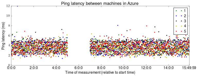
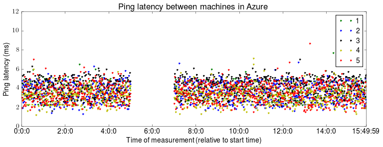
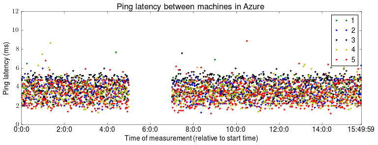
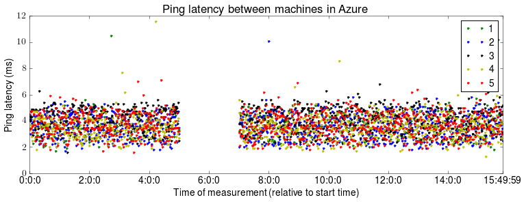
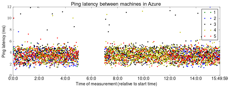
The following 5 plots show the RTT as observed by each machine over time. The y axis stops as 12 ms to aid visibility of the majority of results. Using the CDF of all results from the second part in this series, we can see that these figures thus include around 85% of all data points.

alt text
alt text
alt text
alt text
alt text

The most striking aspect of these figures is the 2 hour gap in the results. The source of this failure is still unknown. Azure reported no machine or network failures during this time and the system removed and continued to take measurements without any manual intervention. Otherwise, between 2 and 5 ms the RTT measurements appear to be fairly randomly distributed, although as we saw last time their distribution approximates normal (as we would expect).

Overall, I am not particularly happy with the results collected so far and hope the next round of tests will generate better results. Tomorrow, we will compare how these results differ from other studies.

Azure Latency Pilot Study: Part 3 – Machine specific results

In this post we will be looking at the results for the Azure latency Pilot study described last week. Yesterday, we started by looking at the aggregated results and found that the measured RTT was larger then expected. Today, we will look at how the results vary depending on which VMs the measurements where taken between. It may be the case that we can infer something about topology between VMs, for example whether VM’s are in the same physical host and the same rack.

The table below shows the RTT between each pair of VMs. The first server in the pair, labelled src is the one which initialised the ping. The table includes each machine pinging itself for comparison.

src dst mean s.d min 25th 50th 75th max
1 1 51.0 65.1 1.7 4.3 65.25 71.6 1004.0
1 2 12.1 89.7 1.7 2.9 3.6 4.3 1004.7
1 3 9.5 66.5 1.6 3.4 4.1 4.8 1004.7
1 4 7.3 52.3 1.3 3.0 3.5 4.0 1004.1
1 5 11.8 84.9 1.6 3.0 3.6 4.4 1242.2
2 1 6.2 12.7 1.6 3.0 3.7 4.425 88.4
2 2 16.7 65.8 1.1 3.0 3.7 4.6 1002.9
2 3 15.0 95.6 1.4 3.0 3.7 4.4 1004.9
2 4 9.6 62.0 1.4 2.9 3.5 4.3 1003.6
2 5 15.3 80.0 1.3 2.9 3.5 4.3 1002.5
3 1 48.5 44.9 2.0 4.5 64.2 70.6 754.9
3 2 7.0 48.9 1.4 2.9 3.6 4.4 1005.0
3 3 3.9 4.2 1.6 3.1 3.8 4.6 124.9
3 4 5.8 32.0 1.3 2.9 3.4 4.0 628.6
3 5 6.7 52.5 1.5 2.9 3.8 4.4 1229.3
4 1 48.8 48.3 1.9 4.7 62.1 67.3 1003.0
4 2 7.7 59.5 1.3 2.8 3.6 4.4 1003.8
4 3 9.0 60.1 1.6 3.3 4.1 4.8 1004.0
4 4 5.2 29.3 1.2 2.7 3.3 3.8 754.6
4 5 15.6 104.7 1.5 2.8 3.6 4.3 1035.0
5 1 50.9 69.8 2.0 4.5 63.8 69.6 1005.3
5 2 9.4 70.9 1.3 2.9 3.7 4.3 1003.8
5 3 8.6 57.6 2.0 3.3 4.1 4.8 1003.7
5 4 6.5 47.7 1.3 2.7 3.4 4.0 1003.0
5 5 6.8 49.2 1.2 2.5 3.2 4.1 1023.0

All VMs other than VM 2 have high latency to VM 1. In fact, we see an average 65 ms RTT from VM 1 to itself. This warrants further investigation into how hping3 is measuring latency. Removing VM 1 from the equation, we observe reasonable uniformity in the RRTs between VMs 2 to 5. Between these the min, 25th, 50th and 75th percentile are all similar and the maximum varies highly, which is to be expected.

I would like to take a close look at how the distribution of RTT measurements varies between VMs 2 to 5. The table below shows the RTT between each pair of VMs between 2 to 5, at various percentile points.

src dst 80th 90th 95th 98th 99th
2 2 5.1 41.8 47.2 124.6 150.7
2 3 4.6 5.0 5.5 34.5 429.5
2 4 4.5 4.9 5.5 47.4 78.5
2 5 4.5 5.4 60.4 91.8 207.8
3 2 4.5 4.8 5.0 5.5 8.9
3 3 4.7 5.0 5.1 5.4 5.8
3 4 4.2 4.5 4.8 5.2 6.1
3 5 4.6 4.9 5.2 5.9 6.6
4 2 4.5 4.8 5.0 5.2 5.8
4 3 5.0 5.2 5.4 5.7 6.4
4 4 4.0 4.3 4.7 5.1 5.8
4 5 4.5 4.8 5.2 6.1 762.9
5 2 4.5 4.8 4.9 5.1 6.1
5 3 4.9 5.2 5.4 5.6 6.8
5 4 4.1 4.5 4.9 5.3 6.3
5 5 4.3 4.6 4.8 5.8 7.2

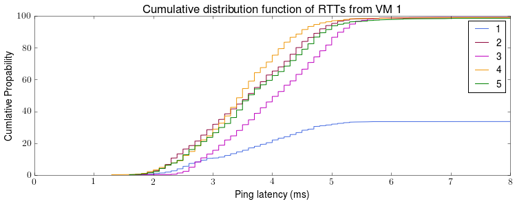
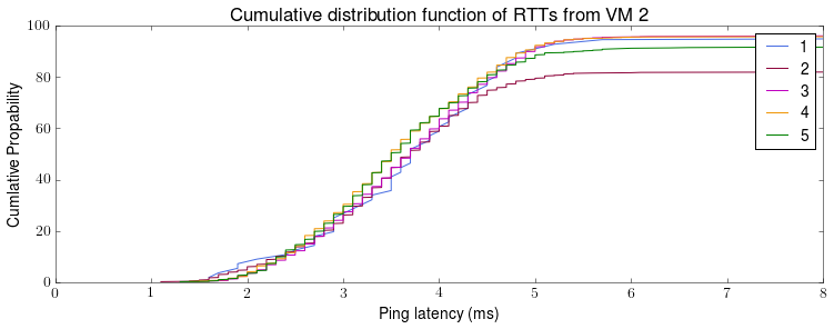
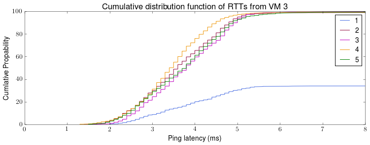
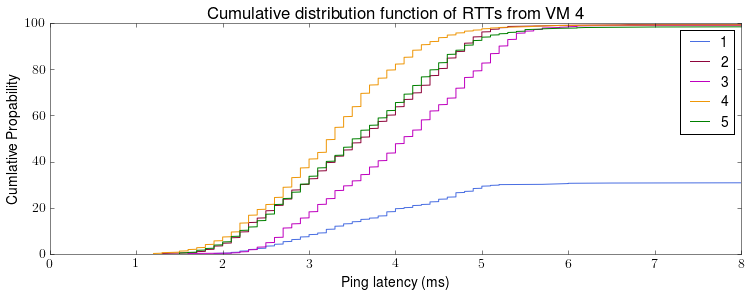
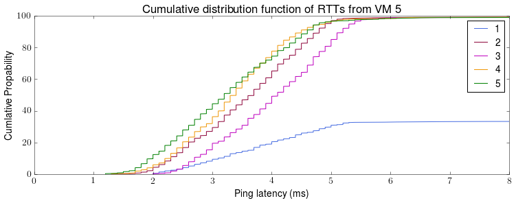
Yesterday, we saw that the 90th percentile for dataset as a whole was 61.4 ms, this is not representative of the RTT between VMs 2-5. We can see this information more clearly using the following 5 CDF, each graph representing the round trip time from each machine to each of the others (and itself).

alt text
alt text
alt text
alt text
alt text

Machine 1 is a clear outlier from the perspective for machines 1, 3, 4 and 5. The observed RTT doesn’t seems to be symmetric. Again this asymmetry warrants further investigation. The stepping in the CDFs is because the RTT is recorded to the nearest 1 decimal place.

Next time, we will look at how the observed RTT varies with time.

Azure Latency Pilot Study: Part 2 – Aggregated results

This is post we will be looking at the results for the Azure latency Pilot study described last week. We will starting by looking at the aggregate results, disregarding the time a measurement was taken and which machines the measurement was taken between.

The 22332 data points have been processed in Python3, in particular using the matplotlib and numpy libraries. The scripts are available in azure-measurements repository.
They currently only use the average round trip time, as reported by hping3, average over 10 pings.

property RTT (ms)
min 1.1
max 1242.2
mean 15.9
std 66.5

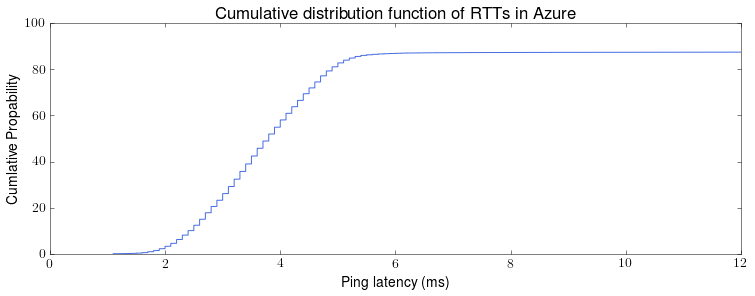
The results in the table above are much larger than I expected. Given the large standard deviation and very large maximum value, it is likely that a few large measures have skewed the results. Let’s take a look at the cumulative distribution function (CDF) and percentile points to see if this is the case.

percentile RTT (ms)
25th 3.0
50th 3.8
75th 4.7
90th 61.4
95th 69.7
99th 87.3

alt text

As expect, some large measurements have skewed the results. However, the proportion of measurement which are considered large is much greater then I expected. This warrants further investigation.

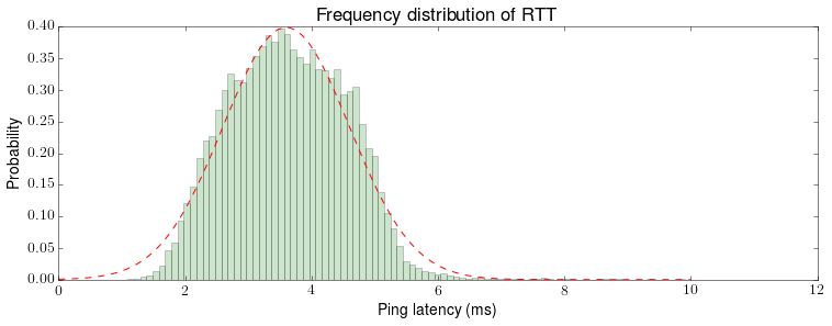
Before that, lets take a closer look at how the majority of value are distributed. Due to the central limit theorem and the sufficiently large sample size, we would expect to see a normal distribution. In simulators such as Raft Refloated, we simulate latency as normally distributed with given parameters, discarding values below a threshold value. We can take a closer look at the probability density function (PDF) and see if this is a reasonable approximation.

alt text

The green bars represent the probability of each RTT. We see an approximate normal distribution, although it is clear that this distribution doesn’t have the same parameters as the data set as a whole. The red lines shows a normal distributed with mean 3.6 and standard deviation of 1. This red line appears to be a reasonable approximation and could be used in simulation.

Next post, we will looks at how the measured RTT differs depending which of the 5 machines the measurement was taken between.

Adding machines can decrease availability of a distributed system

TL;DR: Run distributed systems using majority quorum on an odd number of machines.

Paxos, Raft, Viewstamped Replication and many other consensus algorithms operate on majority quorums. A majority quorum is any subset of nodes containing at least a strict majority of nodes. These algorithms all require a majority quorum to agree to a value before its considered to be committed. This ensures that any agreement will be aware of all past agreements, as there will always be in intersection of at least one mode between any two majority quorums.

It is a prerequisite that at least a strict majority of nodes are up for the system using these consensus protocols to be operational. From this, we can establish an upper bound on the uptime of any system using majority quorum consensus. For this calculation, we assume node failures are independent. Whilst this is a fair assumption, it is of course not the case in practice.

We can calculate the probability that a strict majority of node are up as follows:

majority_bound_fig2

p is the probably that a node is live, n is number of nodes and underline means floor.

This equation is also the CDF of the Binomial distribution. It works by summing up the probability what no nodes are down, only one node is down, two nodes are down etc.. until you reach the case where the largest possible minority of nodes are down.

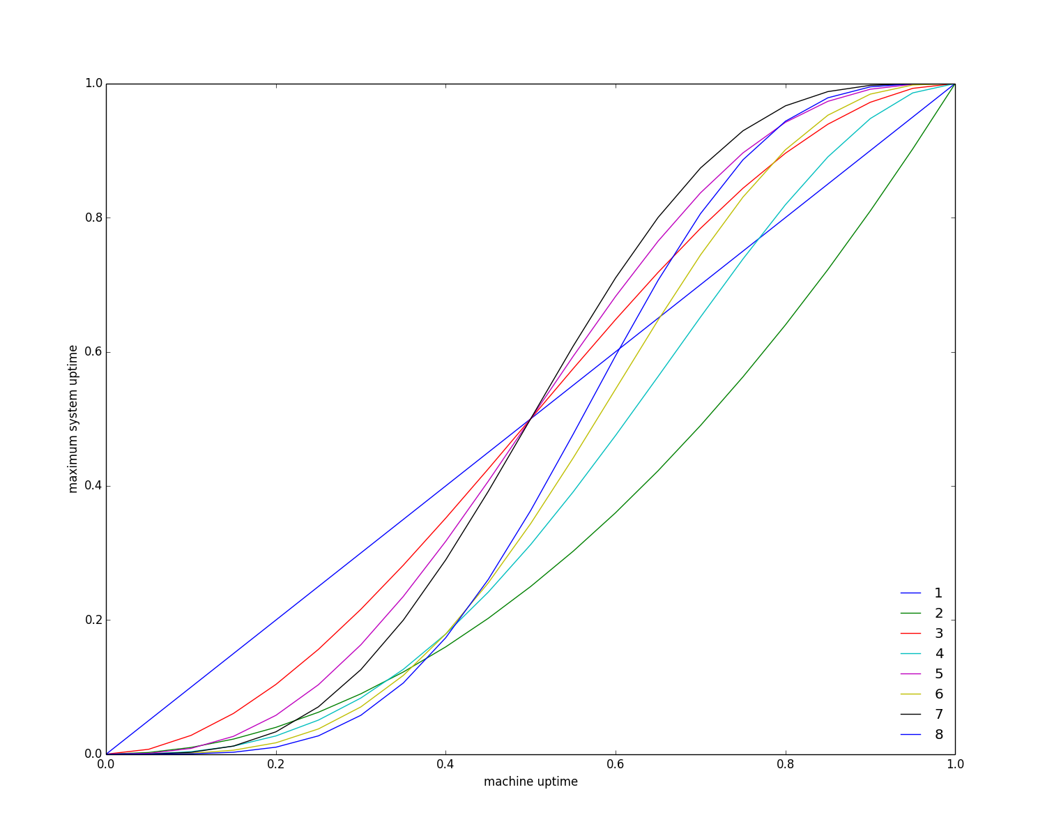
The following graph shows the relationship between node uptime p and majority quorum uptime (each line represent the number of nodes from 1 to 8):

majority_bound_fig1

A system with two nodes is more likely to fail than a system with one. It’s easy to see why this is. If either node in a system of two machines fails then the system is down (as its unable to get a strict majority). Since there are two node instead of one, a failure is likely to occur. In other words, the probably of a system of one node having a majority is p, whilst for a system of two nodes its p^2.

If node uptime is less than half, your best off with only one node. In practice, your best off with not using majority quorum consensus.

Adding a node to an odd set of nodes doesn’t improve uptime. Adding this extra node doesn’t increase the number of failures that can we handled, e.g. 5 nodes can handle upto two failures and 6 nodes can also only handle upto two failures. The summation above has no extra terms in this case but the existing terms are smaller as p is raised to a higher power.

This approach is of course very limited. We are not accounting for how extra nodes aid in the handling of read-only commands, the duration and pattern of failures and that machine failures are not independent.

I assume this is well known result in the theory of distributed system but I’ve not come across it before. If anyone has seen it before, I can you send me a pointer to the work.

Chronicle of Coracle: Parsing Protocol Specific Parameters

This is the first post in the “Chronicle of Coracle” series to document daily life using OCaml for systems programming.

Today, I’ll be adding protocol specific parameters to Coracle, this mostly involves working with the Yojson and Cmdliner libraries. Once completed, Coracle will be able to accept JSON files like:

{"nodes": 50,"loss": 0.0, "termination":1000, "consensus": {"protocol":"raft","timeout":300}}

Stage 1 – Protocol selection

The value associated with “protocol” key determines how which consensus protocol is ran by the simulator. Though this value seems like an unusual starting place, the simulator is a functor over the specific consensus implementation, thus we much choose our consensus implementation first before anything else. We extract the protocol name as follows:

let get_protocol filename = try (
  Safe.from_file filename
  |> function `Assoc config -> config
  |> List.assoc "consensus"
  |> function `Assoc proto -> proto
  |> List.assoc "protocol" 
  |> function `String str -> str
  |> function "raft" -> `Raft | "vrr" -> `VRR
  ) with _ -> raise JSON_parsing_failure

This approach gets the job done but could be improved using some kinda option/error monad instead of exceptions and providing more detailed information to the user on why the JSON parsing failed. We added various other JSON parsing functions, all of follow a similar pattern one above. We needed to do a bit more work to get these to type correctly, as described in Stage 3.

Stage 2 – The dummy module

Based on the protocol given in the JSON configuration file, we apply a different consensus module to the simulation functor. At the moment we only have support for the Raft protocol, so here is the type sig for consensus modules and a new dummy consensus module we can use in testing.

module type CONSENSUS = sig
  
type state
type config
val parse_config: json -> config
val init: id list -> config -> state
val add_peers: id list -> state -> state
val state_to_string: state -> string 

type msg
val msg_serialize: msg -> string
val msg_deserialize: string -> msg
val msg_to_string: msg -> string
val eval: msg input -> state -> state option * msg output list  

end 

And the dummy module:

open Common
open Io
open Yojson.Safe

type state = {
  peers: id list;
  counter: int;
  say_hello_to: int;
}

type config = int
let parse_config json = 
  function `Assoc config -> config
  |> List.assoc "id"
  |> function `Int i -> i

let init peers id = {
  peers; counter=0; say_hello_to=id}
let add_peers new_peers s = 
  {s with peers=s.peers@new_peers}
let state_to_string s = string_of_int s.counter

type msg = Hello | HelloBack
let msg_to_string = function
  | Hello -> "hello"
  | HelloBack -> "hello back"

let msg_serialize = msg_to_string

let msg_deserialize = function
  | "hello" -> Hello
  | "hello back" -> HelloBack

let eval event state =
  match event with
  | PacketArrival (id,Hello) -> 
(None, [PacketDispatch (id, HelloBack)])
  | PacketArrival (_,HelloBack) -> 
(Some {state with counter=state.counter +1}, [])
  | Startup _ -> 
(None, [PacketDispatch (state.say_hello_to, Hello)])

This was just a quick hack to test that the simulator will generalise over consensus implementations.

Stage 3 – Using mli files to generalise polymorphic variants

Yojson uses polymorphic variants for describing the structure of JSON files. Polymorphic variants (the ones which start with the backtick) can be declared on the fly and don’t need type definitions beforehand. Initially, we got type errors like this for many of our JSON parsing functions:

Error: Signature mismatch:
       ...
       Values do not match:
         val parse_config :
           [< `Assoc of (string * [> `Int of int ]) list ] -> config
       is not included in
         val parse_config : Yojson.Safe.json -> config

These issues where quickly address by adding mli files or :json type annotations


Stage 4 – Knowing when to give up

The simulation command line interface (without using config files) had become exponentially more complex, both in terms of implementation and usage. As of this PR, we on longer support command line simulation without the use of a config file. In hindsight, its unlikely that many would use this interface due to the unmanageable number of parameters (around 2 dozen for ocaml-raft)

Stage 5 – Protocol Selector

Now that we are able to parse the JSON config files and we have multiple protocols to choice between, we can write our protocol selector:

let protocol_selector config_file trace output_file no_sanity =
  match Json_handler.get_protocol config_file with
  | `Raft -> 
    let module R = Simulator.Simulate(Raft) in 
    R.start config_file trace output_file no_sanity
  | `Dummy -> 
    let module R = Simulator.Simulate(Dummy) in 
    R.start config_file trace output_file no_sanity

Since we only have two protocols to choose between, I’ve opted to duplicate the R.start line instead of using first class modules (fcm) as fcm requires packing and unpacking. Interestingly, I can’t directly call start from Simulator.Simulate(Raft), you need to assign it to an intermediate module in between. I’m not sure why this is case.

Conclusion

You can now pass protocol specific parameter to Coracle using JSON configuration files. This will be live on the demo server by tonight. Tomorrow, we will look at adding clients to the simulator.
#C3S2015 Trip Report – Day 0

Hello from a lovely little spa hotel in a forest in Estonia.

After an excellent dinner and many coffees, our first session started at 9pm (yes! they are working us hard already). We received a warm welcome from Olaf Meaneel (TUT) to the first ever cyber security summer school (C3S2015). Dr Parag Pruthi kicked off proceedings with his talk titled “Advancing big data analytics – cyber defence solutions”.

Parag asked “When was the first cyber war?” The answer: in 1982, during the cold war, the CIA attacked the flow control software for soviet serbian gas pipeline. Our networks are even more fragile. Example of Iran hijacking US drone and some excellent clips from the IT crowd. Breaching systems is fast, discovery is slow and recovery is very slow. We always blame ‘dave’, we aren’t good at protecting against human error. Intrusion detection systems are not reliable, 1% false positive rate gives a trust levels of .19%.

We researchers are disconnected from the real world, we make simplifying assumptions, design a solution and test in simulation against the assumptions. Parag motivates engineering from real world network. He details the challenges in collecting petabytes of data, storage, compression, retrieval, processing and evaluating.

Parag key message was that big data provides us with near perfect information for intrusion detection.

Q: Is you approach limited in time, we must collect data and anaylsis before we can react?
A: Correct, we still have real people watching data visualisation, like a security guard watch CCTV, but they are not an order of magnitude faster then they where before.

Paper Notes: Ethical Privacy Guidelines for Mobile Connectivity Measurements [Report Nov’13]

Ethical Privacy Guidelines for Mobile Connectivity Measurements is the first item on the C3S reading list, below is my brief notes on this November 2013 report by the Oxford Internet Institute.

The stated purpose of this report is to inform networking researchers about the best practices for preserving data subject privacy when performing active measurement of mobile networks.

Researcher must make a comprise between the privacy of data subjects and dissemination of research artefacts for reproducibility. To aid in reasoning about this comprise, the report presents a risk assessments format covering: the contributions of the research, risk of de-identification, impact of re-identification, unforeseen risk (such as data theft), methods to dissemination artefacts, informed consent and transparency. The report goes onto discuss a few legal implications, in particular, the ongoing debate on whether IP addresses and communication metadata are personally identifiable information.

The authors focus on a guiding principle: collect the minimal data possible to conducted the stated research. Data should n0t be used for a secondary purpose unless explained at the consent stage. This includes open dissemination of the data collected. The report suggests some methods of fuzzing the data including: perturbation, truncation, permutation, quantisation, pseudonymization, k-anonymity and differential privacy.

Overall, I would recommend the report to someone new to the domain of data privacy, as its a nice introduction to the topic.  The authors raise awareness of the necessary compromise between reproducible research and data privacy. Though they do not provide concrete advise to researchers on how to make the best compromise (other than telling them to be conservative). The report claims to focus on active mobile measurements, in practice its contribution is much more general than this. I would love to see this report with real-world examples of measurement studies that have been conducted, the comprise between reproducible research and data privacy that was chosen and how it was chosen.

Paper Notes: The Network is Reliable [ACMQ July’14]

The Network is Reliable is an excellent article which attempts to formalise the discussion on real world failures for distributed systems. There is currently great debate on whether the assumption that network partitions are rare is too strong or too weak, for modern networks. Much of the data which we could use to answer this question is not published, instead is takes the form of anecdotes shared between sysadmins over a beer. This article lets the reader sit at the table and share the stories.

It is worth noting that network partition is used here in the broadest possible sense. We are looking at end-to-end communications and anything which can hinder these. This goes beyond simple link and switch failures to distributed GC, bugs in the NIC, and slow IO.

Here 5 examples of the anecdotes covered:

  • split brain caused by non-transitive reachability on EC2
  • redundancy doesn’t always prevent link failure
  • asymmetric reachability due to bugs in the NIC
  • GC and blocking for  I/O can cause huge runtime latencies
  • short transient failures become long term problem with existing algorithms

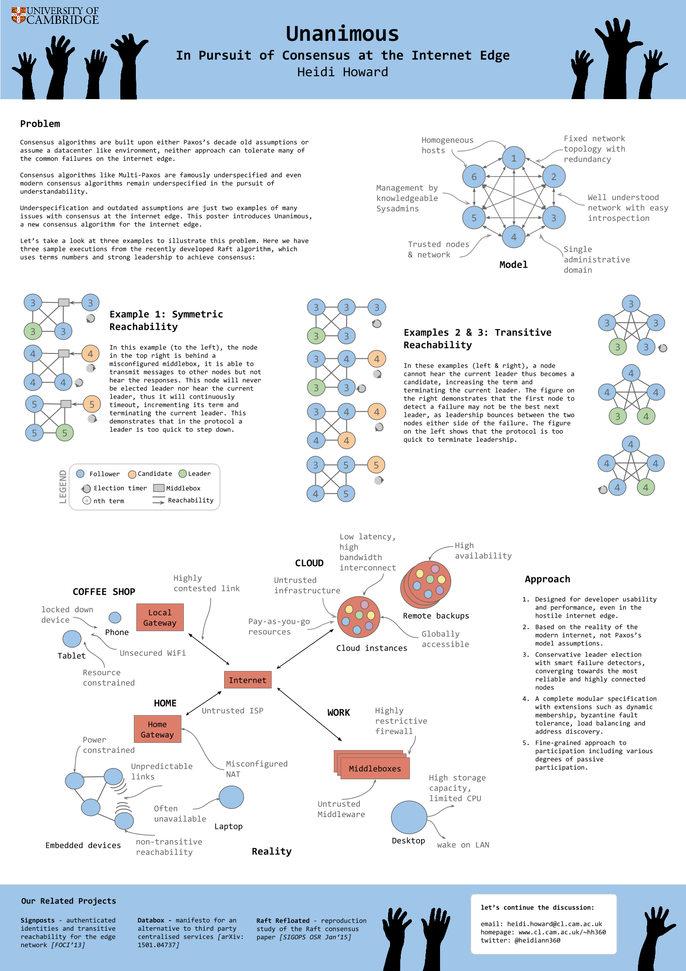
So, what does this mean for Unanimous and my research on reliable consensus for real world networks?

My original inspiration for working on consensus algorithms was the need for reliable consensus at the internet edge. With consensus comes fault tolerance,  from this we can construct new systems for preserving privacy and handling personal data, offering users a viable alternative to 3rd party centralised services.

However, it has become apparent that the issues of reliable consensus is much more general. This article illustrates that even within the constrained setting of a datacenter, distributed systems are failing to tolerance the wide range of possible failures.